The Cassandra Architecture

Jeff Carpenter, Eben Hewitt - Cassandra The Definitive Guide, Third Edition Distributed Data at Web Scale - O’Reilly Media (2022)

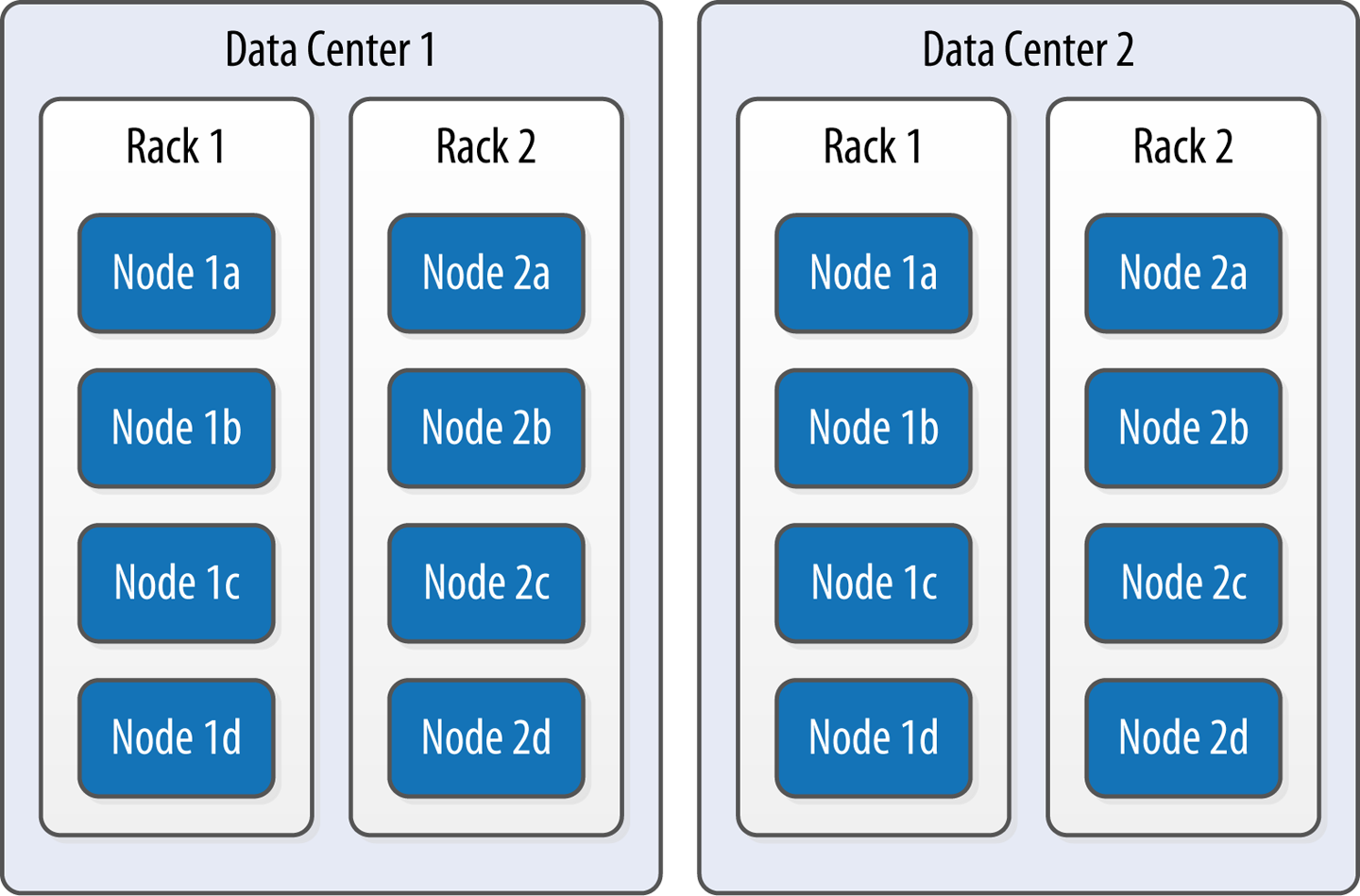
Data Centers and Racks

Gossip and Failure Detection

To support decentralization and partition tolerance, Cassandra uses a gossip protocol that allows each node to keep track of state information about the other nodes in the cluster. The gossiper runs every second on a timer.

Gossip protocols (sometimes called epidemic protocols) generally assume a faulty network, are commonly employed in very large, decentralized network systems, and are often used as an automatic mechanism for replication in distributed databases. They take their name from the concept of human gossip, a form of communication in which peers can choose with whom they want to exchange information.

The gossip protocol in Cassandra is primarily implemented by the org.apache.cassandra.gms.Gossiper class, which is responsible for managing gossip for the local node. When a server node is started, it registers itself with the gossiper to receive endpoint state information.

Because Cassandra gossip is used for failure detection, the Gossiper class maintains a list of nodes that are alive and dead.

Here is how the gossiper works:

1. Once per second, the gossiper will choose a random node in the cluster and initialize a gossip session with it. Each round of gossip requires three messages.

2. The gossip initiator sends its chosen friend a GossipDigestSyn message.

3. When the friend receives this message, it returns a GossipDigestAck message.

4. When the initiator receives the ack message from the friend, it sends the friend a GossipDigestAck2 message to complete the round of gossip.

When the gossiper determines that another endpoint is dead, it “convicts” that endpoint by marking it as dead in its local list and logging that fact.

Cassandra has robust support for failure detection, as specified by a popular algorithm for distributed computing called Phi Accrual Failure Detector. This manner of failure detection originated at the Advanced Institute of Science and Technology in Japan in 2004.

Accrual failure detection is based on two primary ideas. The first general idea is that failure detection should be flexible, which is achieved by decoupling it from the application being monitored. The second and more novel idea challenges the notion of traditional failure detectors, which are implemented by simple “heartbeats” and decide whether a node is dead or not dead based on whether a heartbeat is received or not. But accrual failure detection decides that this approach is naive, and finds a place in between the extremes of dead and alive—a suspicion level.

Therefore, the failure monitoring system outputs a continuous level of “suspicion” regarding how confident it is that a node has failed. This is desirable because it can take into account fluctuations in the network environment. For example, just because one connection gets caught up doesn’t necessarily mean that the whole node is dead. So suspicion offers a more fluid and proactive indication of the weaker or stronger possibility of failure based on interpretation (the sampling of heartbeats), as opposed to a simple binary assessment.

Snitches

The job of a snitch is to provide information about your network topology so that Cassandra can efficiently route requests. The snitch will figure out where nodes are in relation to other nodes. The snitch will determine relative host proximity for each node in a cluster, which is used to determine which nodes to read and write from.

As an example, let’s examine how the snitch participates in a read operation. When Cassandra performs a read, it must contact a number of replicas determined by the consistency level. In order to support the maximum speed for reads, Cassandra selects a single replica to query for the full object, and asks additional replicas for hash values in order to ensure the latest version of the requested data is returned. The snitch helps to help identify the replica that will return the fastest, and this is the replica that is queried for the full data.

The default snitch (the SimpleSnitch) is topology unaware; that is, it does not know about the racks and data centers in a cluster, which makes it unsuitable for multiple data center deployments. For this reason, Cassandra comes with several snitches for different network topologies and cloud environments, including Amazon EC2, Google Cloud, and Apache Cloudstack.

The snitches can be found in the package org.apache.cassandra.locator. Each snitch implements the IEndpointSnitch interface. We’ll learn how to select and configure an appropriate snitch for your environment in Chapter 10.

While Cassandra provides a pluggable way to statically describe your cluster’s topology, it also provides a feature called dynamic snitching that helps optimize the routing of reads and writes over time. Here’s how it works. Your selected snitch is wrapped with another snitch called the DynamicEndpointSnitch. The dynamic snitch gets its basic understanding of the topology from the selected snitch. It then monitors the performance of requests to the other nodes, even keeping track of things like which nodes are performing compaction. The performance data is used to select the best replica for each query. This enables Cassandra to avoid routing requests to replicas that are busy or performing poorly.

The dynamic snitching implementation uses a modified version of the Phi failure detection mechanism used by gossip. The badness threshold is a configurable parameter that determines how much worse a preferred node must perform than the best-performing node in order to lose its preferential status. The scores of each node are reset periodically in order to allow a poorly performing node to demonstrate that it has recovered and reclaim its preferred status.

Rings and Tokens

So far we’ve been focusing on how Cassandra keeps track of the physical layout of nodes in a cluster. Let’s shift gears and look at how Cassandra distributes data across these nodes.

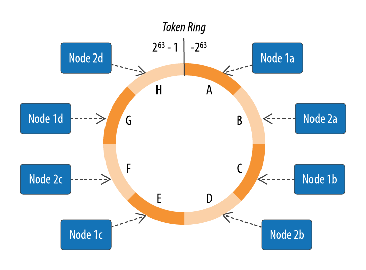
Cassandra represents the data managed by a cluster as a ring. Each node in the ring is assigned one or more ranges of data described by a token, which determines its position in the ring. For example, in the default configuration, a token is a 64-bit integer ID used to identify each partition. This gives a possible range for tokens from −2^63 to 2^63−1. We’ll discuss other possible configurations under “Partitioners”.

A node claims ownership of the range of values less than or equal to each token and greater than the last token of the previous node, known as a token range. The node with the lowest token owns the range less than or equal to its token and the range greater than the highest token, which is also known as the wrapping range. In this way, the tokens specify a complete ring. Figure 6-2 shows a notional ring layout including the nodes in a single data center. This particular arrangement is structured such that consecutive token ranges are spread across nodes in different racks.

Data is assigned to nodes by using a hash function to calculate a token for the partition key. This partition key token is compared to the token values for the various nodes to identify the range, and therefore the node, that owns the data. Token ranges are represented by the org.apache.cassandra.dht.Range class.

To see an example of tokens in action, let’s revisit our user table from Chapter 4. The CQL language provides a token() function that we can use to request the value of the token corresponding to a partition key, in this case the last_name:

cqlsh:my_keyspace> SELECT last_name, first_name, token(last_name) FROM user;

 last_name | first_name | system.token(last_name)
-----------+------------+-------------------------
 Rodriguez |       Mary |    -7199267019458681669
     Scott |     Isaiah |     1807799317863611380
    Nguyen |       Bill |     6000710198366804598
    Nguyen |      Wanda |     6000710198366804598

(5 rows)

As you might expect, we see a different token for each partition, and the same token appears for the two rows represented by the partition key value “Nguyen.”

Virtual Nodes

Early versions of Cassandra assigned a single token (and therefore by implication, a single token range) to each node, in a fairly static manner, requiring you to calculate tokens for each node. Although there are tools available to calculate tokens based on a given number of nodes, it was still a manual process to configure the initial_token property for each node in the cassandra.yaml file. This also made adding or replacing a node an expensive operation, as rebalancing the cluster required moving a lot of data.

Cassandra’s 1.2 release introduced the concept of virtual nodes, also called vnodes for short. Instead of assigning a single token to a node, the token range is broken up into multiple smaller ranges. Each physical node is then assigned multiple tokens. Historically, each node has been assigned 256 of these tokens, meaning that it represents 256 virtual nodes (although we’ll discuss possible changes to this value in Chapter 10). Virtual nodes have been enabled by default since 2.0.

Vnodes make it easier to maintain a cluster containing heterogeneous machines. For nodes in your cluster that have more computing resources available to them, you can increase the number of vnodes by setting the num_tokens property in the cassandra.yaml file. Conversely, you might set num_tokens lower to decrease the number of vnodes for less capable machines.

Cassandra automatically handles the calculation of token ranges for each node in the cluster in proportion to their num_tokens value.(Cassandra 自动处理集群中每个节点的令牌范围计算，与它们的“num_tokens”值成比例Cassandra 自动处理集群中每个节点的令牌范围计算，与它们的“num_tokens”值成比例) Token assignments for vnodes are calculated by the org.apache.cassandra.dht.tokenallocator.ReplicationAwareTokenAllocator class.

A further advantage of virtual nodes is that they speed up some of the more heavyweight Cassandra operations such as bootstrapping a new node, decommissioning(退役) a node, and repairing a node. This is because the load associated with operations on multiple smaller ranges is spread more evenly across the nodes in the cluster.

Partitioners

A partitioner determines how data is distributed across the nodes in the cluster. As we learned in Chapter 4, Cassandra organizes rows in partitions. Each row has a partition key that is used to identify the partition to which it belongs. A partitioner, then, is a hash function for computing the token of a partition key. Each row of data is distributed within the ring according to the value of the partition key token. As shown in Figure 6-3, the role of the partitioner is to compute the token based on the partition key columns.

Any clustering columns that may be present in the primary key are used to determine the ordering of rows within a given node that owns the token representing that partition.

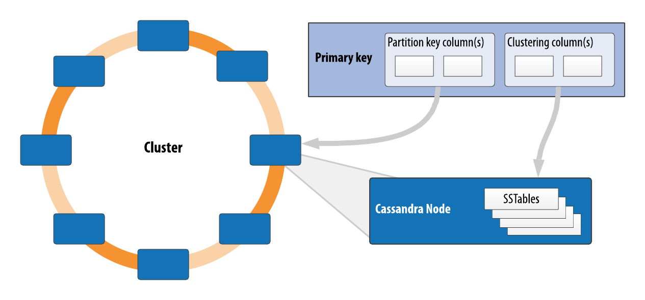
Figure 6-3. The role of the partitioner

Cassandra provides several different partitioners in the org.apache.cassandra.dht package (DHT stands for distributed hash table). The Murmur3Partitioner was added in 1.2 and has been the default partitioner since then; it is an efficient Java implementation on the murmur algorithm developed by Austin Appleby. It generates 64-bit hashes. The previous default was the RandomPartitioner.

Because of Cassandra’s generally pluggable design, you can also create your own partitioner by implementing the org.apache.cassandra.dht.IPartitioner class and placing it on Cassandra’s classpath. Note, however, that the default partitioner is not frequently changed in practice, and that you can’t change the partitioner after initializing a cluster.

Replication Strategies

A node serves as a replica for different ranges of data. If one node goes down, other replicas can respond to queries for that range of data. Cassandra replicates data across nodes in a manner transparent to the user, and the replication factor is the number of nodes in your cluster that will receive copies (replicas) of the same data. If your replication factor is 3, then three nodes in the ring will have copies of each row.

The first replica will always be the node that claims the range in which the token falls, but the remainder of the replicas are placed according to the replication strategy (sometimes also referred to as the replica placement strategy).

For determining replica placement, Cassandra implements the Gang of Four strategy pattern, which is outlined in the common abstract class org.apache.cassandra.locator.AbstractReplicationStrategy, allowing different implementations of an algorithm (different strategies for accomplishing the same work). Each algorithm implementation is encapsulated inside a single class that extends the AbstractReplicationStrategy.

Out of the box, Cassandra provides two primary implementations of this interface (extensions of the abstract class): SimpleStrategy and NetworkTopologyStrategy. The SimpleStrategy places replicas at consecutive nodes around the ring, starting with the node indicated by the partitioner. The NetworkTopologyStrategy allows you to specify a different replication factor for each data center. Within a data center, it allocates replicas to different racks in order to maximize availability. The NetworkTopologyStrategy is recommended for keyspaces in production deployments, even those that are initially created with a single data center, since it is more straightforward to add an additional data center should the need arise.

Legacy Replication Strategies

A third strategy, OldNetworkTopologyStrategy, is provided for backward compatibility. It was previously known as the RackAwareStrategy, while the SimpleStrategy was previously known as the RackUnawareStrategy. NetworkTopologyStrategy was previously known as DataCenterShardStrategy. These changes were effective in the 0.7 release.

The strategy is set independently for each keyspace and is a required option to create a keyspace, as we saw in Chapter 4.

Consistency Levels

In Chapter 2, we discussed Brewer’s CAP theorem, in which consistency, availability, and partition tolerance are traded off against one another. Cassandra provides tuneable consistency levels that allow you to make these trade-offs at a fine-grained level. You specify a consistency level on each read or write query that indicates how much consistency you require. A higher consistency level means that more nodes need to respond to a read or write query, giving you more assurance that the values present on each replica are the same.

For read queries, the consistency level specifies how many replica nodes must respond to a read request before returning the data. For write operations, the consistency level specifies how many replica nodes must respond for the write to be reported as successful to the client. Because Cassandra is eventually consistent, updates to other replica nodes may continue in the background.

The available consistency levels include ONE, TWO, and THREE, each of which specify an absolute number of replica nodes that must respond to a request. The QUORUM consistency level requires a response from a majority of the replica nodes. This is sometimes expressed as:

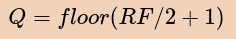
In this equation, Q represents the number of nodes needed to achieve quorum for a replication factor RF. It may be simpler to illustrate this with a couple of examples: if RF is 3, Q is 2; if RF is 4, Q is 3; if RF is 5, Q is 3, and so on.

The ALL consistency level requires a response from all of the replicas. We’ll examine these consistency levels and others in more detail in Chapter 9.

Consistency is tuneable in Cassandra because clients can specify the desired consistency level on both reads and writes. There is an equation that is popularly used to represent the way to achieve strong consistency in Cassandra: R + W > RF = strong consistency. In this equation, R, W, and RF are the read replica count, the write replica count, and the replication factor, respectively; all client reads will see the most recent write in this scenario, and you will have strong consistency. As we discuss in more detail in Chapter 9, the recommended way to achieve strong consistency in Cassandra is to write and read using the QUORUM or LOCAL_QUORUM consistency levels.

Distinguishing Consistency Levels and Replication Factors

If you’re new to Cassandra, it can be easy to confuse the concepts of replication factor and consistency level. The replication factor is set per keyspace. The consistency level is specified per query, by the client. The replication factor indicates how many nodes you want to use to store a value during each write operation. The consistency level specifies how many nodes the client has decided must respond in order to feel confident of a successful read or write operation. The confusion arises because the consistency level is based on the replication factor, not on the number of nodes in the system

Queries and Coordinator Nodes

Let’s bring these concepts together to discuss how Cassandra nodes interact to support reads and writes from client applications. Figure 6-4 shows the typical path of interactions with Cassandra.

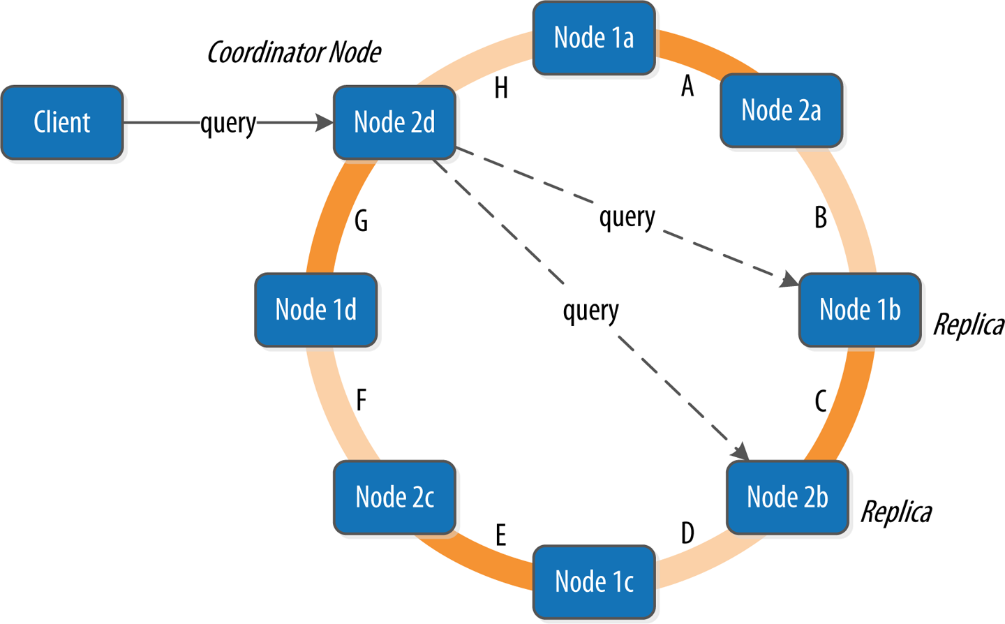
A client may connect to any node in the cluster to initiate a read or write query. This node is known as the coordinator node. The coordinator identifies which nodes are replicas for the data that is being written or read and forwards the queries to them.

For a write, the coordinator node contacts all replicas, as determined by the consistency level and replication factor, and considers the write successful when a number of replicas commensurate with the consistency level acknowledge the write.

For a read, the coordinator contacts enough replicas to ensure the required consistency level is met, and returns the data to the client.

These, of course, are the “happy path” descriptions of how Cassandra works. In order to get a full picture of Cassandra’s architecture, we’ll now discuss some of Cassandra’s high availability mechanisms that it uses to mitigate failures, including hinted handoff and repair.

Hinted Handoff(提示切换)

注解：即是 redo log 重放

Consider the following scenario: a write request is sent to Cassandra, but a replica node where the write properly belongs is not available due to network partition, hardware failure, or some other reason. In order to ensure general availability of the ring in such a situation, Cassandra implements a feature called hinted handoff.

You might think of a hint as a little Post-it Note that contains the information from the write request. If the replica node where the write belongs has failed:

1. the coordinator will create a hint, which is a small reminder that says, “I have the write information that is intended for node B. I’m going to hang on to this write, and I’ll notice when node B comes back online; when it does, I’ll send it the write request.”

2. That is, once it detects via gossip that node B is back online, node A will “hand off” to node B the “hint” regarding the write. Cassandra holds a separate hint for each partition that is to be written.

This allows Cassandra to be always available for writes, and generally enables a cluster to sustain the same write load even when some of the nodes are down. It also reduces the time that a failed node will be inconsistent after it does come back online.

In general, hints do not count as writes for the purposes of consistency level. The exception is the consistency level ANY, which was added in 0.6. This consistency level means that a hinted handoff alone will count as sufficient toward the success of a write operation. That is, even if only a hint was able to be recorded, the write still counts as successful. Note that the write is considered durable, but the data may not be readable until the hint is delivered to the target replica.

There is a practical problem with hinted handoffs (and guaranteed delivery approaches, for that matter): if a node is offline for some time, the hints can build up considerably on other nodes. Then, when the other nodes notice that the failed node has come back online, they tend to flood that node with requests, just at the moment it is most vulnerable (when it is struggling to come back into play after a failure). To address this problem, Cassandra limits the storage of hints to a configurable time window. It is also possible to disable hinted handoff entirely.

As its name suggests, org.apache.cassandra.hints.HintsService is the class that implements hinted handoffs internally.

Although hinted handoff helps increase Cassandra’s availability, due to the limitations mentioned it is not sufficient on its own to ensure consistency of data across replicas.

Anti-Entropy, Repair, and Merkle Trees

Cassandra uses an anti-entropy protocol as an additional safeguard to ensure consistency. Anti-entropy protocols are a type of gossip protocol for repairing replicated data. They work by comparing replicas of data and reconciling differences observed between the replicas. Anti-entropy is used in Amazon’s Dynamo, and Cassandra’s implementation is modeled on that (see Section 4.7 of the Dynamo paper).

Replica synchronization is supported via two different modes known as read repair and anti-entropy repair.

Read repair refers to the synchronization of replicas as data is read. Cassandra reads data from multiple replicas in order to achieve the requested consistency level, and detects if any replicas have out-of-date values.

• If an insufficient number of nodes have the latest value, a read repair is performed immediately to update the out-of-date replicas.

• Otherwise, the repairs can be performed in the background after the read returns. This design is observed by Cassandra as well as by straight key-value stores such as Project Voldemort and Riak.

Anti-entropy repair (sometimes called manual repair) is a manually initiated operation performed on nodes as part of a regular maintenance process. This type of repair is executed by using a tool called nodetool, as we’ll learn about in Chapter 12. Running nodetool repair causes Cassandra to execute a validation compaction (see “Compaction”). During a validation compaction, the server initiates a TreeRequest/TreeReponse conversation to exchange Merkle trees with neighboring replicas. The Merkle tree is a hash representing the data in that table. If the trees from the different nodes don’t match, they have to be reconciled (or “repaired”) to determine the latest data values they should all be set to. This tree comparison validation is the responsibility of the org.apache.cassandra.service.reads.AbstractReadExecutor class.

Lightweight Transactions and Paxos

//TODO

Memtables, SSTables, and Commit Logs

Now let’s take a look inside a Cassandra node at some of the internal data structures and files, summarized in Figure 6-5. Cassandra stores data both in memory and on disk to provide both high performance and durability. In this section, we’ll focus on Cassandra’s storage engine and its use of constructs called memtables, SSTables, and commit logs to support the writing and reading of data from tables.

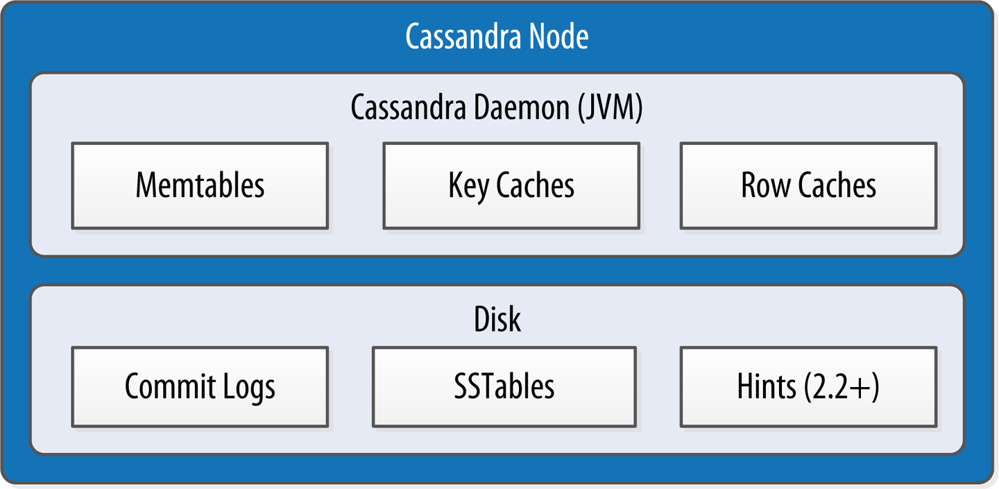
Figure 6-5. Internal data structures and files of a Cassandra node

When a node receives a write operation, it immediately writes the data to a commit log. The commit log is a crash-recovery mechanism that supports Cassandra’s durability goals. A write will not count as successful on the node until it’s written to the commit log, to ensure that if a write operation does not make it to the in-memory store (the memtable, discussed in a moment), it will still be possible to recover the data. If you shut down the node or it crashes unexpectedly, the commit log can ensure that data is not lost. That’s because the next time you start the node, the commit log gets replayed. In fact, that’s the only time the commit log is read; clients never read from it.

After it’s written to the commit log, the value is written to a memory-resident data structure called the memtable. Each memtable contains data for a specific table. In early implementations of Cassandra, memtables were stored on the JVM heap, but improvements starting with the 2.1 release have moved some memtable data to native memory, with configuration options to specify the amount of on-heap and native memory available. This makes Cassandra less susceptible to fluctuations in performance due to Java garbage collection. Optionally, Cassandra may also write data to in memory caches, which we’ll discuss in “Caching”.

When the number of objects stored in the memtable reaches a threshold, the contents of the memtable are flushed to disk in a file called an SSTable. A new memtable is then created. This flushing is a nonblocking operation; multiple memtables may exist for a single table, one current and the rest waiting to be flushed. They typically should not have to wait very long, as the node should flush them very quickly unless it is overloaded.

Why Are They Called “SSTables”?

The term “SSTable” originated in Google Bigtable as a compaction of “Sorted String Table.” Cassandra borrows this term even though it does not store data as strings on disk.

Each commit log maintains an internal bit flag to indicate whether it needs flushing. When a write operation is first received, it is written to the commit log and its bit flag is set to 1. There is only one bit flag per table, because only one commit log is ever being written to across the entire server. All writes to all tables will go into the same commit log, so the bit flag indicates whether a particular commit log contains anything that hasn’t been flushed for a particular table. Once the memtable has been properly flushed to disk, the corresponding commit log’s bit flag is set to 0, indicating that the commit log no longer has to maintain that data for durability purposes. Like regular log files, commit logs have a configurable rollover threshold, and once this file size threshold is reached, the log will roll over, carrying with it any extant dirty bit flags.

Once a memtable is flushed to disk as an SSTable, it is immutable and cannot be changed by the application. Despite the fact that SSTables are compacted, this compaction changes only their on-disk representation; it essentially performs the “merge” step of a mergesort into new files and removes the old files on success.

Since the 1.0 release, Cassandra has supported the compression of SSTables in order to maximize use of the available storage. This compression is configurable per table.

All writes are sequential, which is the primary reason that writes perform so well in Cassandra. No reads or seeks of any kind are required for writing a value to Cassandra because all writes are append operations. This makes the speed of your disk one key limitation on performance. Compaction is intended to amortize the reorganization of data, but it uses sequential I/O to do so. So the performance benefit is gained by splitting; the write operation is just an immediate append, and then compaction helps to organize for better future read performance. If Cassandra naively inserted values where they ultimately belonged, writing clients would pay for seeks up front.

On reads, Cassandra will read both SSTables and memtables to find data values, as the memtable may contain values that have not yet been flushed to disk. Memtables are implemented by the org.apache.cassandra.db.Memtable class.

Bloom Filters

Bloom filters are used to boost the performance of reads.

//TODO

Caching

As an additional mechanism to boost read performance, Cassandra provides three optional forms of caching:

• The key cache stores a map of partition keys to row index entries, facilitating faster read access into SSTables stored on disk. The key cache is stored on the JVM heap.

• The row cache caches entire rows and can greatly speed up read access for frequently accessed rows, at the cost of more memory usage. The row cache is stored in off-heap memory.

• The chunk cache was added in the 3.6 release to store uncompressed chunks of data read from SSTable files that are accessed frequently. The chunk cache is stored in off-heap memory.

• The counter cache was added in the 2.1 release to improve counter performance by reducing lock contention for the most frequently accessed counters.

By default, key and counter caching are enabled, while row caching is disabled, as it requires more memory. Cassandra saves its caches to disk periodically in order to warm them up more quickly on a node restart. We’ll investigate how to tune these caches in Chapter 13.

Compaction

As we already discussed, SSTables are immutable, which helps Cassandra achieve such high write speeds. However, periodic compaction of these SSTables is important in order to support fast read performance and clean out stale data values. A compaction operation in Cassandra is performed in order to merge SSTables. During compaction, the data in SSTables is merged: the keys are merged, columns are combined, obsolete values are discarded, and a new index is created.

Compaction is the process of freeing up space by merging large accumulated datafiles. This is roughly analogous to rebuilding a table in the relational world. But the primary difference in Cassandra is that it is intended as a transparent operation that is amortized across the life of the server.

On compaction, the merged data is sorted, a new index is created over the sorted data, and the freshly merged, sorted, and indexed data is written to a single new SSTable (each SSTable consists of multiple files, including Data, Index, and Filter). This process is managed by the class org.apache.cassandra.db.compaction.CompactionManager.

Another important function of compaction is to improve performance by reducing the number of required seeks. There is a bounded number of SSTables to inspect to find the column data for a given key. If a key is frequently mutated, it’s very likely that the mutations will all end up in flushed SSTables. Compacting them prevents the database from having to perform a seek to pull the data from each SSTable in order to locate the current value of each column requested in a read request.

When compaction is performed, there is a temporary spike in disk I/O and the size of data on disk while old SSTables are read and new SSTables are being written.

Cassandra supports multiple algorithms for compaction via the strategy pattern. The compaction strategy is an option that is set for each table. The compaction strategy extends the AbstractCompactionStrategy class. The available strategies include:

• SizeTieredCompactionStrategy (STCS) is the default compaction strategy and is recommended for write-intensive(密集的) tables.

• LeveledCompactionStrategy (LCS) is recommended for read-intensive tables.

• TimeWindowCompactionStrategy (TWCS) is intended for time series or otherwise date-based data.

We’ll revisit these strategies in Chapter 13 to discuss selecting the best strategy for each table.

One interesting feature of compaction relates to its intersection with incremental repair. A feature called anticompaction was added in 2.1. As the name implies, anticompaction is somewhat of an opposite operation to regular compaction in that the result is the division of an SSTable into two SSTables, one containing repaired data, and the other containing unrepaired data.

The trade-off is that more complexity is introduced into the compaction strategies, which must handle repaired and unrepaired SSTables separately so that they are not merged together.

Deletion and Tombstones

We’ve already discussed several common distributed system approaches that Cassandra uses to handle failure gracefully. Another interesting case has to do with deleting data. Because a node could be down or unreachable when data is deleted, that node could miss a delete. When that node comes back online later and a repair occurs, the node could “resurrect” the data that had been previously deleted by re-sharing it with other nodes.

To prevent deleted data from being reintroduced, Cassandra uses a concept called a tombstone. A tombstone is a marker that is kept to indicate data that has been deleted. When you execute a delete operation, the data is not immediately deleted. Instead, it’s treated as an update operation that places a tombstone on the value.

A tombstone is similar to the idea of a “soft delete” from the relational world. Instead of actually executing a delete SQL statement, the application will issue an update statement that changes a value in a column called something like “deleted.” Programmers sometimes do this to support audit trails, for example.

Tombstones are not kept forever; instead, they are removed as part of compaction. There is a setting per table called gc_grace_seconds (Garbage Collection Grace Seconds), which represents the amount of time that nodes will wait to garbage collect (or compact) tombstones. By default, it’s set to 864,000 seconds, the equivalent of 10 days. Cassandra keeps track of tombstone age, and once a tombstone is older than gc_grace_seconds, it will be garbage collected. The purpose of this delay is to give a node that is unavailable time to recover; if a node is down longer than this value, then it should be treated as failed and replaced.

Managers and Services

Cassandra Daemon

Storage Engine

Cassandra’s core data storage functionality is commonly referred to as the storage engine, which consists primarily of classes in the org.apache.cassandra.db package. The main entry point is the ColumnFamilyStore class, which manages all aspects of table storage, including commit logs, memtables, SSTables, and indexe

Storage Service

Cassandra wraps the storage engine with a service that is represented by the org.apache.cassandra.service.StorageService class. The storage service contains the node’s token, which is a marker indicating the range of data that the node is responsible for.

The server starts up with a call to the initServer method of this class, upon which the server registers the thread pools used to manage various tasks, makes some determinations about its state (such as whether it was bootstrapped or not, and what its partitioner is), and registers an MBean with the JMX server.

Storage Proxy

The org.apache.cassandra.service.StorageProxy sits in front of the StorageService to handle the work of responding to client requests. It coordinates with other nodes to store and retrieve data, including storage of hints when needed. The StorageProxy also helps manage lightweight transaction processing.

Messaging Service

The purpose of org.apache.cassandra.net.MessagingService is to manage all inbound and outbound messages from this node to and from other nodes, except for SSTable streaming, which we’ll examine next. Incoming messages are routed to the other services referenced in this section for handling. Outgoing messages may optionally have callbacks, which are invoked when a response is received from the other node.

Stream Manager

Streaming is Cassandra’s optimized way of sending SSTable files from one node to another via a persistent TCP connection; all other communication between nodes occurs via serialized messages. Streaming may occur when tokens need to be reallocated across the cluster, such as when a node is added or removed. Streaming may also occur during repair processing or when a node is being replaced or rebuilt. We’ll learn more about these operations in [Chapter 12](javascript:void(0)).

The org.apache.cassandra.streaming.StreamManager handles these streaming messages, including connection management, message compression, progress tracking, and statistics.