Connection tracking (conntrack) - Part 2: Core Implementation#
With this article series I like to take a closer look at the connection tracking subsystem of the Linux kernel, which provides the basis for features like stateful packet filtering and NAT. I refer to it as the “ct system” throughout the series. In this second article, I take a deep look under the hood and dive into its core implementation. I revisit some of the topics of the first article, but this time on source code level. I give an overview of the most important data structures and explain how handling of the connection tracking table, connection lookup and connection life cycle works.
Articles of the series#
The ct table#
The ct system maintains the connections which it is tracking in a central table. A very time efficient lookup into that table is essential, because it needs to be performed for nearly every network packet which comes along. Thus, it is implemented as a hash table.
Quick refresher on Hash Tables
A hash table is by definition an associative array, a data structure which maps keys to values. It is useful in cases where the keys themselves are too complex to simply directly be used as integer indices in an array, because the theoretical total number of all possible keys would be too huge. These keys could e.g. be text strings specifying the name of a person and the values could be address- or customer-records of that person. Thus, when doing a lookup for a value based on a key, the approach is to calculate a simple hash from the key, whose range of possible values is small enough so that it can be used as index in an array (e.g. a hash size of 8bit which results in an array size of 2^8=256 entries). The advantage here is that hash calculation as well as index lookup in the array can both be performed in a constant amount of time, which means algorithmic complexity O(1). The obvious disadvantage is, that due to the limited number range of the hash, collisions are unavoidable (different keys having the same hash). Thus, each entry in the array of the hash table (each “bucket”) does not just contain a single value, but instead a doubly linked list of all values which match (“collide”) to this hash. This means, that algorithmic complexity of the lookup is at best O(1) and at worst O(n): After the hash calculation and array index, the doubly linked list of that bucket needs to be traversed to find the correct value for the key in question. This further implies, that the key needs to be saved inside (as part of) the value itself, because this is the only means a comparison can be done to find it.
Obviously three relevant actions can be performed with this table: A lookup can be performed on the table to find an existing tracked connection corresponding to a network packet. A new connection instance can be added to the table. And a connection can be removed from the table, e.g. when the connection “expires”. The ct system maintains an individual timer/timeout for each connection to let it “age” and “expire”, which results in its removal and deletion sooner or later, depending on the situation. It is interesting to note, that the ct table actually is a central table, which means only one table exists for the whole system and not one table per network namespace(ct table 居然是所有 network namespaces 共享同一个的!). To avoid hash collisions for similar traffic in different network namespaces, a namespace-specific seed hash_mix1) is used during hash calculation. To further ensure reliable distinction, each tracked connection instance possesses a reference to the network namespace it belongs to. That reference is additionally being checked on connection lookup.
Hash table keys: tuples#
In case of the ct system, the keys for the hash table need to be something that can be easily extracted from the layer 3 and 4 protocol headers of a network packet and which clearly indicates to which connection that packet belongs to. The ct system calls those keys “tuples” and implements them in form of the data type struct nf_conntrack_tuple. Function nf_ct_get_tuple() is used to extract the required data from the protocol headers of a network packet and then fill the member variables of an instance of that data type with values. Figure 1 shows this based on an example TCP packet.
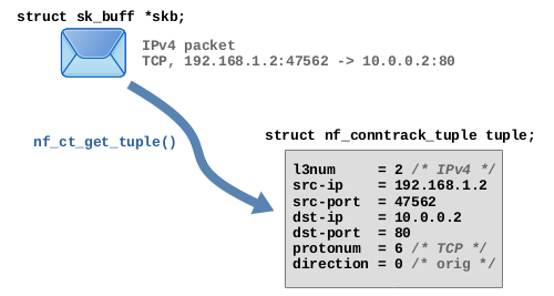
Figure 1: A tuple is being created from an example TCP packet
In case of TCP, a tuple roughly spoken contains the source and destination IP addresses plus the TCP source and destination ports which together represent both endpoints of the connection. The data type struct nf_conntrack_tuple is flexible enough to hold extracted protocol header data of several different layer 3 and 4 protocols. Some of its members are implemented as union types which are able to contain different things depending on the protocols. Semantically the data type contains the following items:
OSI Layer 3
Protocol number: 2 (IPv4) or 10 (IPv6)
Source IP address
Destination IP address
OSI Layer 4
Protocol number: 1 (ICMP)2)/ 6 (TCP)/ 17 (UDP)/ 58 (ICMPv6)/ 47 (GRE)/ 132 (SCTP)/ 33 (DCCP)
Protocol-specific data
TCP/UDP: source port and destination port
ICMP: type, code and identifier
…
Direction: 0 (orig) / 1 (reply)
Hash table values: struct nf_conn#
Let’s take a look at the values in the hash table, the tracked connections, which are implemented as instances of struct nf_conn. That structure is a little more complex, possesses quite a list of member variables and can even be extended dynamically during runtime, depending on the layer 4 protocol and depending on several possible extensions. Figure 2 shows a simplified view of the structure with the member variables, which I consider most relevant regarding the scope of this article. As you can see, it contains:
a reference counter,
a timeout to handle expiration,
a reference to the network namespace to which that connection belongs to,
an integer for status bits of that connection and layer 4 protocol-specific data.
In case of TCP the latter e.g. contains things like tracked TCP sequence numbers and so on.
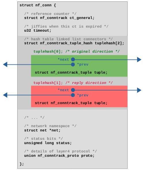
Figure 2: Simplified view of
struct nf_connwith most relevant member variables.
A very interesting member is the tuplehash[2] array, which is the means by which instances of struct nf_conn are being integrated into the hash table. As mentioned, it is necessary in hash tables to save the key (here, the tuple struct nf_conntrack_tuple) as part of the value (here, struct nf_conn), because the lookup in the hash table will only work by comparing keys, if the hash has collisions. However, in case of the ct system, there is one more bit of complexity to add here: It must be possible to do the lookup of a tracked connection in the hash table for network packets which flow in the original data flow direction and also for packets which flow in the reply direction. Both will result in different tuples and different hashes, but a lookup must still find the same instance of struct nf_conn in the end. For this reason, tuplehash is an array with two elements. Both elements each contain a tuple and pointers3) to connect this element to the linked list of a “bucket” of the hash table. The first element, shown in green color in Figure 2, represents the original direction. The member direction of its tuple is set to 0 (orig). The second element, shown in red color in Figure 2, represents the reply direction. The member direction of its tuple is set to 1 (reply). Of course only one instance of struct nf_conn exists for each tracked connection, but that instance is being added twice to the hash table, once for the original direction and once for the reply direction, to make lookups for both kind of packets possible. I’ll describe that in detail below.
Lookup existing connection#
Let’s walk through the connection lookup in detail. In Figure 3 a TCP packet is traversing the ct hook function in the Netfilter Prerouting hook4). Most of the interesting part of that hook function is done in function nf_conntrack_in(). Among other functions, it calls resolve_normal_ct() and this is where the lookup happens. Figure 3 shows that in detail. In this example I assume that the connection the TCP packet belongs to is already known and tracked by the ct system at this point. In other words, I assume that this is not the first packet of that connection which the ct system is seeing.
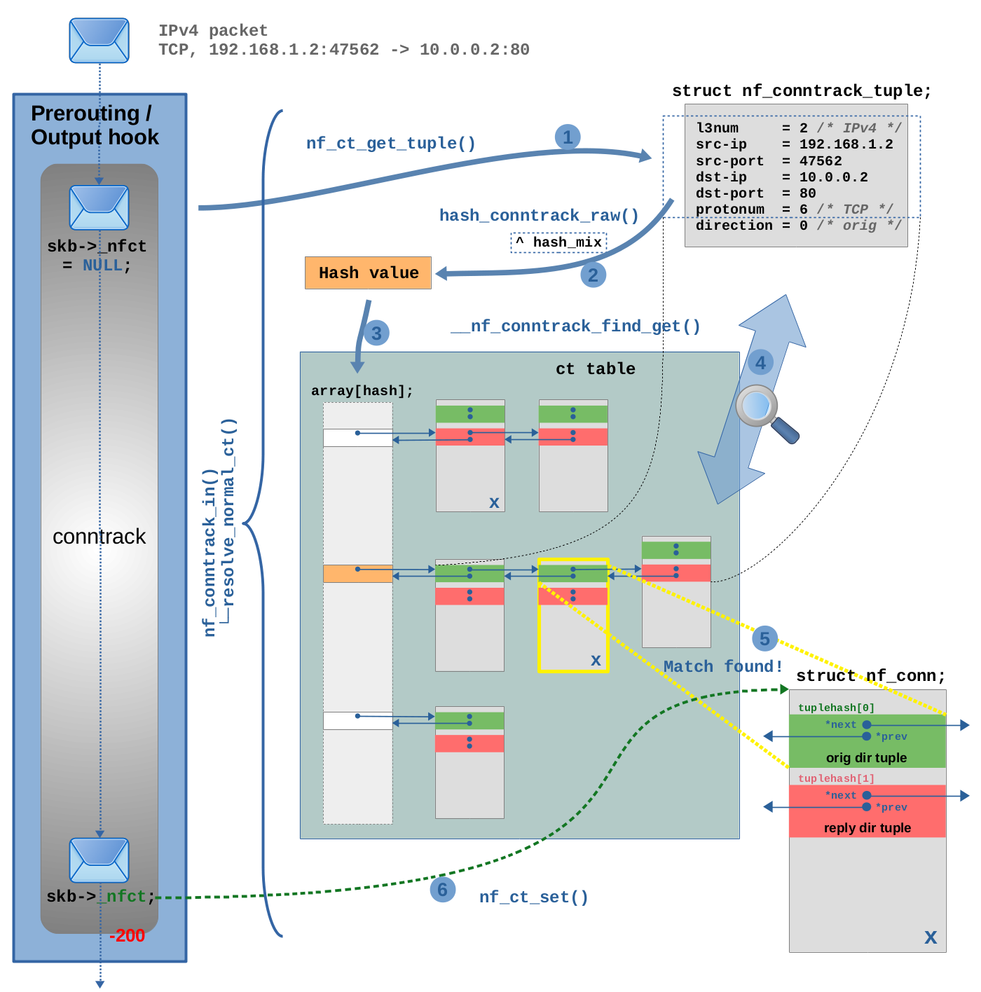
Figure 3: Lookup of tracked connection in detail
In step (1) function nf_ct_get_tuple() is called to create a tuple, the key to the hash table, from the TCP packet (same thing as already shown in Figure 1). Member direction of the tuple is always set to 0 (orig) in this case. It has no real meaning here, because at this point it is yet unknown to the ct system, whether the TCP packet is part of the original or the reply direction of a tracked connection. In step (2) function hash_conntrack_raw() is called to calculate the hash value from the member variable values of the tuple. Member direction is not included in the hash calculation, as the dotted rectangle in Figure 3 indicates, for the reason just explained. However, the mentioned seed hash_mix of the network namespace is additionally included. Now the actual lookup in the hash table is performed by function __nf_conntrack_find_get() in steps (3), (4) and (5): The hash value is used as index in the array of the hash table in step (3) to locate the correct bucket, as shown in orange color in Figure 3. In this example that bucket already contains three instances of struct nf_conn. In other words, three tracked connections here already collide for this hash. In step (4) the code now iterates through the linked list of this bucket and compares the tuple inside the member tuplehash[] of each connection instance with the tuple which has been generated from the TCP packet in step (1). A connection is considered a match, if all member variables of the tuple match (except member direction, which is ignored here again) and further, the network namespace matches. A match is found in step (5). I marked the matching instance with an X in Figure 3 to show that it exists in two different places within the hash table. In one place it is connected to the bucket linked list with the pointers of its tuplehash[0] member (original direction, shown in green color) and in another place it is connected with the pointers of its tuplehash[1] member (reply direction, shown in red color). As you can see, it is tuplehash[0] (green) which matches in step (5). This means the TCP packet in question is part of the original direction of this tracked connection. In step (6) function nf_ct_set() is called to initialize skb->_nfct of the network packet to point to the just found matching instance of struct nf_conn5). Finally now the OSI layer 4 protocol of the packet (in our example TCP) is being examined6), before the packet finishes traversing the ct hook function.
Adding a new connection#
But what happens if the lookup described above does not produce a match? In that case the TCP packet will considered to be the very first packet of a new connection which is not yet being tracked by the ct system. Function resolve_normal_ct() will call init_conntrack() to create a new instance of a tracked connection. Figure 4 shows how this works.
 Figure 4: Creating a new connection instance
At first, two tuples are created to cover both data flow directions. The first one, named orig_tuple and shown in green color in Figure 4, actually is the one which has already been created by function nf_ct_get_tuple() during the connection lookup described above in step (1) of Figure 3. It is simply being re-used here. I just show this here again as step (1) of Figure 4 to visualize all the relevant data in one place. The orig_tuple represents the original data flow direction and its member direction is set to 0 (orig). This is by definition always the data flow direction of the very first packet of that connection which is seen by the ct system, in this case 192.168.1.2:47562 -> 10.0.0.2:80. In step (2) function nf_ct_invert_tuple() is called. It creates a second tuple, the reply_tuple, shown in red color in Figure 4. This one represents the reply data flow direction, 10.0.0.2:80 -> 192.168.1.2:47562 in this case. Its member direction is set to 1 (reply). Function nf_ct_invert_tuple() does not create it based on the TCP packet. It uses orig_tuple as input parameter. This action would even work both ways. You could always use nf_ct_invert_tuple() to create a tuple of the opposite data flow direction based on an existing tuple. In this example, what it does is quite simple, because we are using TCP. Function nf_ct_invert_tuple() here simply flips source and destination IP addresses and source and destination TCP ports. However, this function is quite intelligent and in case of other protocols it does other things. E.g. in case of ICMP, if the orig_tuple would describe an ICMP echo-request (type=8, code=0, id=42), then the inverted reply_tuple would describe and echo-reply (type=0, code=0, id=42). In step (3) a new instance of struct nf_conn is allocated and its members are initialized. The two tuples both become part of it. They are inserted in the tuplehash array. Several more things happen here… expectation check, extensions… I won’t go into all the details. This new instance of a tracked connection is still considered “unconfirmed” at this point and thus in step (4) it is being added to the so-called unconfirmed list. That is a linked list which exists per network namespace and per CPU core. Step (5) is the exact same thing as step (6) in Figure 3 during the lookup, initializing skb->_nfct of the network packet to point to the new connection instance. Finally now the OSI layer 4 protocol of the packet (in our example TCP) is being examined7), before the packet finishes traversing the ct hook function. In this example here I assume that the network packet is not being dropped while it continues on its way through the kernel network stack and through one or more potential Nftables chains and rules. Finally, the packet traverses one of the conntrack “help+confirm” functions (the ones with priority MAX). Inside it, the new connection will get “confirmed” and be added to the actual ct hash table. This is shown in detail in Figure 5.
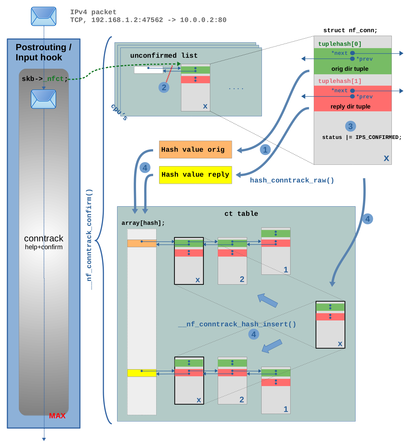 Figure 5: Confirming the new connection instance and adding it to the ct hash table
The interesting part of the code is located in function __nf_conntrack_confirm(). This code is only executed if the tracked connection belonging to this network packet (our example TCP packet) is yet “unconfirmed”. This is determined by checking the IPS_CONFIRMED_BIT bit in the status member of struct nf_conn, which is 0 at this point. In step (1) both hashes are calculated, one from the orig_tuple and another from the reply_tuple within the struct nf_conn instance8). Then in step (2) the instance of struct nf_conn is being removed from the unconfirmed list. In step (3) the IPS_CONFIRMED_BIT is set to 1 in the status member, “confirming” it. Finally in step (4) the instance is being added to the ct table. The hashes are used as array indices to locate the correct buckets. Then the struct nf_conn instance is added to the linked lists of both buckets, one time with its tuplehash[0] for the orig direction and another time with its tuplehash[1] for the reply direction.
Removing a connection#
Removing a connection instance from the ct table obviously means removing it from the linked lists of both buckets where it resides within the table. This is done in function clean_from_lists(). However, this does not yet delete that particular connection instance. There is more to say about deletion. I’ll get to that below.
Connection life cycle, reference counting#
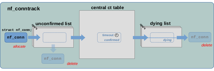 Figure 6: Life cycle9) of a tracked connection instance
In the following sections I will take a more detailed look at the life cycle of tracked connections, which I already explained shortly in the previous article; see Figure 6. Internally, that life cycle is being handled via reference counting. Each instance of struct nf_conn possesses its own reference counter struct nf_conntrack ct_general (see Figure 2). That structure contains an atomic_t integer named use. When a struct nf_conn instance is being added to the ct table, use is incremented by 1 and decremented by 1 when the instance is being removed from the table. For every network packet, which references to an instance of struct nf_conn with its member skb->_nfct, use is incremented by 1 and decremented by 1 when the skb is being released10). The ct system’s API provides functions for incrementing/decrementing use. Function nf_conntrack_get() increments it and function nf_conntrack_put() decrements it. The declaration of struct nf_conn contains a comment which states that reference counting behavior and if you review the code carefully, you’ll be able to confirm it. However, a little warning ahead… the overall code handling the struct_nf_conn reference counting is a little hard to read, because those two functions are not being used everywhere. In some places the integer use is instead being modified by other functions11).
Connection deletion#
When function nf_conntrack_put() decrements the reference counter use to zero, then it calls nf_conntrack_destroy(), which deletes the instance of struct nf_conn. It does that by means of a whole bunch of sub functions. Those call nf_ct_del_from_dying_or_unconfirmed_list(), which does exactly what its name suggests, and then call nf_conntrack_free(), which does the actual deletion or “de-allocation”. In other words, the code assumes that struct nf_conn instance is currently either on the unconfirmed list or on the dying list by the time the reference counter use is decremented to zero. If you look at Figure 6, then you see that those actually are the only two situations when deletion is supposed to occur: When a connection instance is on the unconfirmed list, deletion can occur if the network packet which triggered its creation is dropped before it reaches the conntrack “help+confirm” hook function. Dropping the packet means the skb is being deleted/freed. Function skb_release_head_state() is part of this deletion and it calls nf_conntrack_put(), which decrements the reference counter use to zero12) and thereby triggers nf_conntrack_destroy(). The other situation where deletion can occur is when a connection instance is on the dying list. But how does it get there in the first place? I’ll get to that, but first I need to explain the timeout mechanism.
Connection timeout#
Once a tracked connection instance is being added to the ct table and marked as “confirmed”, a timeout is set for it to “expire” somewhen in the near future, if no further network packet of that connection arrives13). This means, usually each further network packet traversing the main ct hook functions which is identified to belong to a tracked connection (=for which the lookup in the ct table finds a match), will cause the timeout of that connection to be resetted/restarted. Thus, a tracked connection won’t expire as long as it stays busy. It will expire, once no further traffic has been detected for some time. How long it takes to expire, strongly depends on the type of the layer 4 protocol and the state. Common expiration timeouts seem to vary in the range from 30 seconds to 5 days. The ct system will e.g. choose a short timeout (by default 120 seconds), when the layer 4 protocol is TCP and the connection currently is in the middle of the TCP 3-way-handshake (If the tracked connection has been created due to a TCP SYN packet and currently the ct system is waiting for TCP SYN ACK on the reply direction…). However, it will choose a long timeout (by default 5 days), once the TCP connection is fully established, because TCP connections can be quite long-living. The default timeout values are hard coded. You can e.g. see them for the TCP protocol being listed in array tcp_timeouts[] in nf_conntrack_proto_tcp.c.
As a system admin you can read and also change/override those default timeout values for your current network namespace via sysctl. The ct system provides the files /proc/sys/net/netfilter/nf_conntrack_*_timeout* for this purpose. The unit of the timeout values in those files is seconds.
A few more words regarding the timeout implementation: The described timeout handling is based on the jiffies software clock mechanism of the kernel. Each instance of struct nf_conn possesses(拥有) an integer member named timeout (see Figure 2). When e.g. a timeout of 30 seconds for a connection shall be set, then this member is simply set to the jiffies value which corresponds to “now” and an offset of 30 * HZ is added. From that moment on, function nf_ct_is_expired() can be used to check for expiration. It simply compares timeout to the current jiffies value of the system.
Quick refresher on “jiffies”
Like countless other kernel components, the ct systems makes use of the “jiffies” software clock mechanism of the linux kernel, which basically is a global integer that is initialized with zero on system boot and is being incremented by one in regular intervals by means of timer interrupts. The interval is defined by build time config variable HZ14), which e.g. on my system (Debian, x86_64) is set to 250, which means jiffies is being incremented 250 times per second and thereby the interval is 4ms. Man page man 7 time gives a short summary.
Do not confuse all this with the timeout extension of the ct system. That extension is some additional and optional mechanism which is implemented on top of the timeout handling described here. It adds even more flexibility, by e.g. allowing to set connection timeouts via Nftables.
GC Workqueue#
But when and how often does the ct system actually check each tracked connection for expiration? Nearly all what I described so far happens within the ct system’s hook functions when network packets traverse those. The idea of the timeout however is to make a tracked connection expire, if no further traffic is detected for some time. Obviously that expiration checking cannot be done in the hook functions. The ct system uses the workqueue mechanism of the kernel to run the garbage collecting function gc_worker in regular intervals within a kernel worker thread15). It moves through the tracked connection instances in the central ct table and checks them for expiration with mentioned function nf_ct_is_expired(). If an expired connection is found, function nf_ct_gc_expired() is called. By means of a whole bunch of sub functions, the IPS_DYING_BIT in the status member of that connection is set, the connection is removed from the central ct table and added to the dying list. Reference counting makes sure, that nf_conntrack_destroy() is called (as already described above). This removes the connection again from the dying list and then finally deletes it.
Thy dying list#
Why is there a dying list at all? By default, the whole garbage collection of a tracked connection… removing it from the ct table, setting the IPS_DYING_BIT, adding it to the dying list, then removing it from the dying list again and finally deleting it… all that by default is done without interruption by the sub functions below nf_ct_gc_expired(). This is why I show a dotted line in the dying list in Figure 6. So one could argue that by default the dying list is not required to exist at all. However, there is a special case, which seems to be the reason for its existence16): This is when you use the userspace tool conntrack with option -E to live view ct events. Here a mechanism comes into play which makes it possible to communicate certain events within the ct system like a new tracked connection being created, a connection being deleted and so on… to userspace. Those operations can potentially block and this is why in this case the latter part of the garbage collection (removing the connection from the dying list and deleting it) needs to be deferred to yet another worker thread in that case. It cannot be allowed that this event mechanism blocks or slows down garbage collection worker thread itself.
Context#
The described behavior and implementation has been observed on a v5.10.19 kernel in a Debian 10 buster system with using Debian backports on amd64 architecture, using kernel build configuration from Debian.